Mathematical models are always wrong, as the famous George Box quotation "All models are wrong, but some are useful" reminds us, but their strength also lies in their stupidity (Smaldino, 2007). Even simple models can make important inferences and predictions despite being quite obviously wrong, such as the simple model of publication bias by John Ioannidis, because the language of mathematics and statistics exposes hypotheses and theories so barely, and constructs numerical predictions about the world so precisely, meaning inferences can be reproduced, expanded, explored, contested and criticised. At a time when the reproducibility crisis spreads to a growing number of disciplines, mathematical modelling is an attractive paradigm, even for disciplines that do not typically engage in formal modelling, because the reproducibility crisis is less about statistics than it is about the absence of strong theory (Green, 2021), and formal mathematical models present about the strongest hypotheses and theories you can find.
For many years, research on shelter and owned dog behaviour has developed a number of practical tests to predict dog behaviour in the future. For shelter dogs, the key estimand is how well a test predicts behaviour post-adoption from the shelter. And in recent years, the value of these standardized tests of behaviour has been questioned, demonstrated by dogs sometimes showing quite different behaviour post-adoption compared to being at the shelter (Marder et al., 2013), and because return rates to shelters seem impervious to whether certain sub-tests are removed from standardized testing protocols.
Ten years ago from the time of writing, Patronek & Bradley (2016) wrote an article arguing that shelter dog behaviour assessments are unlikely to be much better than 'flipping a coin', because test sensitivity and specificity are likely moderate to low, and the prior probability of problematic behaviours, like aggression, are already relatively rare in the companion dog population. They presented a mathemtical model of diagnostic testing, which indicated that even with relatively optimistic values of test sensitivity and specificity, a positive shelter dog test for aggression would only indicate a 50% chance that the dog is actually 'aggressive'.
The model of diagnostic testing employed in Patronek & Bradley (2016) is another example of an elementary Bayesian model. It is the same model, more or less, considered by Ioannidis in his model of publication bias, and it is the same model I have played around on this blog before. Because it's simple, it's also easily breakable, and because we can break it, we might be able to find ways to improve the predicability of tests of shelter dog behaviour.
Think of a dog undergoing a test of food aggression in a shelter, where the dog is given a bowl of food and is approached by a tester, perhaps with a plastic, fake hand on a stick, which will be used to touch the dog and even enter the food bowl while the dog is eating. The simple model assumes a pass/fail on the test, where a positive test (denoted by $+$) is recorded if the dog shows any growling, snarling or snapping towards the tester or fake hand, and a negative (denoted by $-$) otherwise. The goal of the test is to measure whether the dog is actually aggressive (A) or non-aggressive (NA) in this context. Bayes' rule, and the simple model of diagnostic testing, tells us that the probability of a dog being aggressive if they have a positive test, $P(A \mid +)$, is:
$$ \begin{align} P(A \mid +) &= \frac{P(+, A)}{P(+)}\\ &= \frac{P(+ \mid A) P(A)}{P(+ \mid A)P(A) + P(+ \mid NA)P(NA)} \end{align} $$This provides us with the posterior probability that a dog is aggressive given a positive test, where $P(A)$ is the marginal or prior or 'pre-study' probability of aggression, $P(+ \mid A)$ is the likelihood of a positive test from an aggressive dog, also known as sensitivity, and $P(+ \mid NA) = 1 - P(- \mid NA)$ is the complement of specificity, the 'false discovery rate', one minus the probability a non-aggressive dog is recorded with a negative test. Plugging in a prior probability of 16%, and optimistic values of sensitivity and specificity of 85% each, Patronek & Bradley (2016) demonstrate that the posterior probability above is only 52%. The argument is that aggression in dogs is relatively rare, probably not more than 1 in 6 dogs, and because the posterior probability is proportional to the likelihood and prior, the prior has a big impact.
The findings of this model are quite compelling, despite it being nothing but a simple application of Bayes' rule. The generative model behind this process is akin to a Bernoulli mixture model, where there is a latent Bernoulli state of aggressive/non-aggressive, and a Bernoulli pass/fail outcome. The causal model assumes that latent aggression status influences behaviour in standardized tests, and the strength of these relationships is captured in the sensitivity and specificity probabilities above. We can write out this generative model explictly as:
$$ \begin{align} \small \theta &= 0.16\\ \pi &= 0.85\\ \gamma &= 0.85\\ p(A \mid \theta) &\sim \mathrm{Bernoulli(\theta)}\\ p(NA \mid \theta) &\sim \mathrm{Bernoulli}(1 - \theta)\\ p(+ \mid A) &\sim \mathrm{Bernoulli}(\pi)\\ p(+ \mid NA) &\sim \mathrm{Bernoulli}(1 - \gamma)\\ \end{align} $$where $\theta$ is now the fixed prior probability of aggression, $\pi$ is now the sensitivity, and $\gamma$ is the specificity, meaning the posterior can be restated as:
$$ \begin{equation} P(A \mid +) = \frac{\pi \theta}{\pi \theta + (1 - \gamma) (1 - \theta)} \end{equation} $$But what happens when we don't just have one test, we have multiple tests of behaviour? That is, the same test has been repeated a number of times. Then we have a sequence of pass/fail outcomes, and we need a different model to compute our posterior probability. Luckily, this is also a well known model, and can be computed using knowledge of sequences of Bernoulli trials. Let's say that we give 2 repeated tests. Naively, we would make the posterior probability of the first test, 52%, be the prior for the next, and run the calculation again, but we can also update the simple Bayes' rule equation above to reflect the posterior probability given a sequence of $k$ positive tests from $n$ total tests:
$$ \begin{equation} \small P(A \mid n, k) = \frac{ \pi^k (1 - \pi)^{n - k} \theta }{ \pi^k (1 - \pi)^{n - k} \theta + (1 - \gamma)^k \gamma^{n - k} (1 - \theta) } \end{equation} $$Plugging $n=2, k=2$ into this equation gives us a considerably larger 86% chance that a dog is aggressive given two positive tests. That's pretty remarkable, and much more useful than flipping a coin. The same model Patronek & Bradley (2016) used to advocate against shelter dog assessments can now be used to advocate for those assessments if we increase the number of tests to two from one. If we get three positives from three tests, we get a whopping 97% chance the dog is aggressive given the data. If we have two tests, and the first is positive and the second is negative, we go from a 52% chance the dog is aggressive given one positive test to 16% that the dog is aggressive after a positive and then a negative test, which is also a lot more helpful than simply flipping a coin. In the formula above, the likelihood is a product of Bernoulli probability mass functions (PMFs), $p^k (1 - p)^{n - k}$ for some probability $p$, but we could also have used the binomial PMF, ${n \choose k} p^k (1 - p)^{n - k}$, and gotten the same answer, providing we don't really care about the order the sequences come in.
Clearly, more tests help, and there are certain shelters employing longitudinal assessments of dog behaviour, where dog behaviour is monitored through time to build a better picture of how they typically behave, a topic I in fact worked on during my PhD (see the preprint Goold & Newberry, 2021 for more details). But let's take a step back and think about the generative process implied by this model. Firstly, $\theta$ should not really be a fixed 16%, because there is uncertainty about its true value. Patronek & Bradley even mention that this is a difficult quantity to estimate. Secondly, the medical diagnostic testing framework assumes that aggression is a simple yes/no, have-it-or-not phenomenon, and that's surely too simplistic. Aggression is likely a spectrum, one of degree and not kind, and every dog will have the ability to be aggressive in the right situation, however rare, in the same way that people will always have a chance of losing their temper, even if that chance is very close to zero.
A first step in the right direction is to take the model above, but rather than assuming a 16% fixed prior on $\theta$, we place a distribution on the prior propensity to show aggression. Let's say that $\theta \sim \mathrm{beta}(\mu \nu, (1 - \mu) \nu)$, which means $\theta$ has a beta distribution, a probability density function (pdf) bounded in the interval (0, 1), with mean $\mu$ and 'sample size' $\nu$. We'll set $\mu = 0.16$ and the $\nu = 50$, which roughly means a 5% chance that the aggression propensity is above 25%, and a ~11% chance aggression propensity is lower than 10%. This means aggression rates are on average 16% with some variation that is not too large or too small. Next, the latent state $z \sim \mathrm{Bernoulli}(\theta)$ represents whether a particular dog being tested has an aggression problem. Yes, for now, this is still discrete. Finally, we have the same likelihood as above, which depends on sensitivity and specificity. The posterior distribution of $p(z = 1 \mid n = 1, k = 1)$ is now more complex:
$$ \begin{equation} p(z = 1 \mid n = 1, k = 1) = \frac{ \mathrm{Binomial}(1 \mid 1, \pi) p(z = 1 \mid \theta) p(\theta) }{ \int_{\theta} \mathrm{Binomial}(1 \mid 1, \pi) p(z = 1 \mid \theta) p(\theta) d\theta } \end{equation} $$I fit this model in Stan, marginalized out the latent state $z$, and calculated $p(z = 1 \mid n = 1, k = 1)$ afterwards. If you're interested in the Stan model, you can see it at the Github repository.
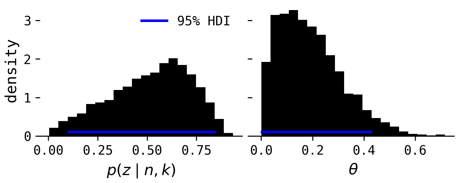
This distribution has a mean of 52% (the same as before), but with a 95% highest density interval (HDI) that ranges from $\sim$10% to $\sim$85%. Therefore, the 'coin flipping' analogy is again not really the whole story. Even with a mildly informative prior distribution, there is considerable uncertainty about the how predictive the test is for future levels of aggression. This raises a second important point: it's not so much that a single test is so unreliable to be useless, it's that a single test is not nearly enough information about a dog to tell us either way if they're likely to show aggression or not.
We could also frame this model assuming a continuous latent state $z$, which represents 'aggressiveness'. Keeping $\theta$ the same, I'll define this latent state as a random normal variable, with its mean a function of $\theta$ and a relatively weakly informative standard deviation of 0.25, $z \sim \mathrm{normal}(\mathrm{logit}(\theta), 0.25)$. Define $z^{*} = \pi \mathrm{logit}^{-1}(z) + (1 - \gamma) \mathrm{logit}^{-1}(z)$, so that a high $z$ has a probability of aggression close to the sensitivity, and a low $z$ has a probability of aggression close to one minus the specificity. I fit this model in Stan, and here are the posterior quantities of interest.
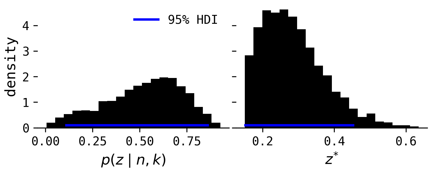
This model doesn't change the results but is a different generative model, whereby $z$ is a latent spectrum, and we only transform it into a probability as a link function for the likelihood. This is somewhat similar to assuming there is a population-level propensity to show aggression, $\theta$, and $z$ is some quantity that depends on the population propensity but is also a noisy filter of it. The variable $z^{*}$ encodes information about sensitivity and specificity, as above. The real value in more complex models will be in training them on datasets of dog aggression, and making inferences about how behaviour changes through time, so we can improve predictions.
There are many more extensions of this model to consider, such as temporal correlation between tests, bias and measurement error, all of which have an impact on the posterior probability of aggression given a series of test results. While Patronek & Bradley (2016)'s article raises important issues, I don't think it's evidence against shelter dog behaviour assessments as much as it's the start of a conversation about what assumptions and formal mathematical modelling can do to help us generate hypotheses and theories about how dog behaviour in shelters changes through time. A key issue is collecting more data about behaviour while dogs are in the shelter, and using repeated tests to improve the precision of our predictions. This isn't necessarily easy, as shelters have limited resources, but it is a way forward, which small expansions of the mathematical model above can help guide.