Earlier this year, I signed up to Hardcover, a book tracking app from a small, independent developer team, working purely for equity and targeting B-corp status. I read a modest amount every year and in the past used Goodreads to record when I had completed each book, but find its interface old and clunky, as do many others. While there are some things I don't love about Hardcover, it's a significantly nicer experience than Goodreads, and it's always nice to support independent developers when possible.
One thing common among book tracking apps, and book review pages, is some kind of Likert scale rating system. Goodreads uses a 1-5 ordinal scale and only recently allowed half- and quarter-star scores. Hardcover also use a 1-5 scale offering half-star scores. Each of these sites aggregates book review scores by taking averages, and although I haven't looked into the algorithms behind book recommendation systems, I'd expect these algorithms treat the Likert scale responses as a type of metric data, that is a continuous scale.
Statistically, there are good reasons why we should not treat book review ratings as metric. Ordinal scores are discrete random variables that do not behave the same way as interval- or ratio-scaled data. Two times a rating of 1 star does not imply 2 stars, for instance, and the distance between 5 and 4 stars might be larger or smaller than the distance between 2 and 3 stars. The appropriate statistical approach to analysing and ranking ordinal response scales is an ordinal data-generating process.
Define $y_{nmp} \in \{1, ..., K\}$ as the $n^{th}$ rating of book $m$ by reader $p$, assumed to have a categorical distribution with category probabilities $\mathbf{\pi}_{nmp}$. The category probabilities are determined by assuming a latent, continuous scale ($z$) underlies the ordinal rating scale, chunked by $K - 1$ thresholds. Each category's probability is the corresponding cumulative density under the curve between those thresholds. The chart below shows the ordered probit model, which assumes the latent scale is distributed $z \sim \mathrm{normal}(\mu, \sigma)$, demonstrated using six different combinations of $\mu$ and $\sigma$.
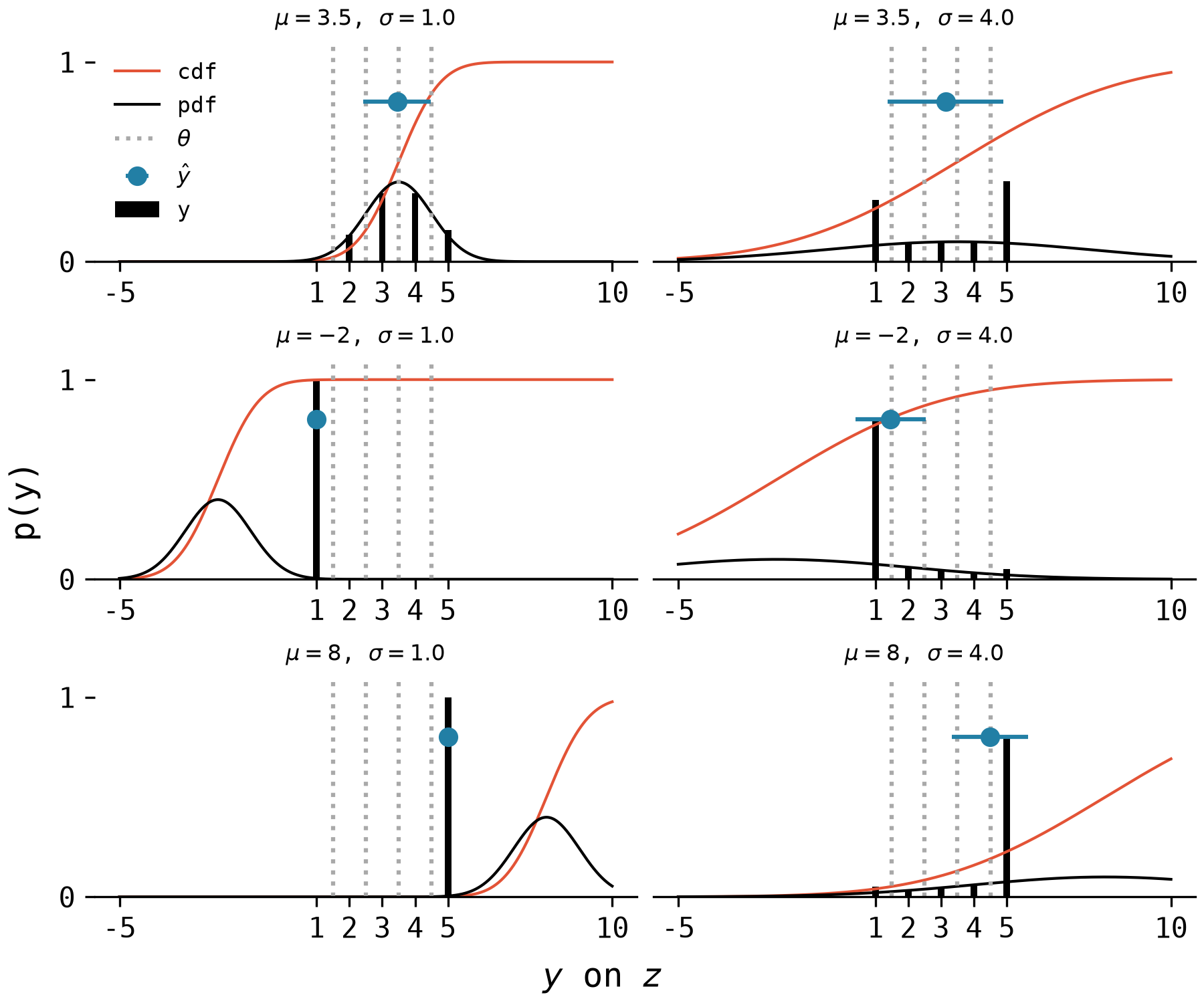
The important thing to realise in these examples is that the distribution of the ordinal responses is not always obvious from the underlying latent distribution, taking a range of shapes depending on the underlying mean and standard deviation of $z$. When $\mu$ sits clearly within the ordinal response categories, and the standard deviation is small, the mean and standard deviation of the ordinal responses themselves are not too dissimilar (the top left panel). However, shifting the mean or widening the standard deviation means the simple descriptive summaries of the ordinal responses themselves will be limited. Most obviously, there are floor and ceiling effects (the middle left and bottom left panels). Liddell & Kruschke (2018) wrote an excellently clear article presenting a range of inferential problems by treating ordinal data as if it was metric. From a prediction perspective, moreover, ordinal models gives us a clear data-generating process by which to simulate new data.
The ordinal data generating process is summarised in the box below.
If you want to play around with this data-generating process, You can simulate your own ordered probit data using the following Python function.
import numpy as np

from scipy.stats import norm

def ordered_probit_rng(
    theta: list[float],
    mu: float,
    sigma: float,
    rng: np.random.Generator | None = None,
    n: int | None = None,
) -> tuple[list[float], list[int]]:
    """Simulate from the ordered-probit model"""

    if rng is None:
        rng = np.random.default_rng()

    K = len(theta) + 1
    thetab = np.array([-np.inf] + [*theta] + [np.inf])

    pi = (
        norm.cdf((thetab[1:] - mu) / sigma) -
        norm.cdf((thetab[:-1] - mu) / sigma)
    )

    if n is None:
        sims = rng.choice(range(1, K + 1, 1), p=pi)
    else:
        sims = rng.choice(range(1, K + 1, 1), size=n, p=pi)
    return pi, sims
Bayesian hierarchical model applied to Goodreads book ratings
I was interested in how book ratings might differ if we applied a suitable ordinal model to Likert ratings rather than just ranked books by the arithmetic average of their ratings. I downloaded FastML's Goodbooks (2017) 10k Goodreads dataset and built a hierarchical ordinal model that accounted for variation across books and users, respectively. Specifically, the ordinal model above is extended to have mean function: $\mu_{nmp} = \alpha + \tau z_{m} + \delta z_{p}$, where $z_{m}$ and $z_{p}$ are standard normal random variates. The full dataset contains 10k books and 6 million ratings, which would take a lot of Bayesian computing time to fit to, so for the purpose of this small blog post I took a 20% sample of ratings from each of the top 100-rated books (determined by total ratings count) as training data, and an additional 100 ratings per book as a test dataset. This amounted to a training data set with $\sim$ 200k ratings over the 100 books. I used Stan to fit the hierarchical ordinal model. You can see the full Stan code on Github, if interested. Here's a small snippet of the model demonstrating the Stan implementation of the ordered probit likelihood.
// snippet of ordered_probit.stan

real ordered_probit_lpmf(int y, real mu, real sigma, vector theta) {
    int J = size(theta);
    int K = J + 1;
    vector[K] pi;
    pi[1] = Phi_approx( (theta[1] - mu) / sigma);
    pi[K] = 1 - Phi_approx( (theta[J] - mu) / sigma);
    pi[2:J] = (
        Phi_approx( (theta[2:J] - mu) / sigma ) -
        Phi_approx( (theta[1:J-1] - mu) / sigma )
    );
    return categorical_lupmf(y | pi);
}
First, let's see how the hierarchical ordinal model compares against some simpler models, in terms of out-of-sample rating performance. Alongside the hierarchical ordinal model, I fit a complete pooling version of the ordered probit model that assumed no variation between books and between users, a hierarchical lognormal regression model with book- and user-varying intercepts that represented an ordinal-as-metric data assumption, and lastly a hierarchical Poisson regression model also with book- and user-varying intercepts, as it's plausible someone might reach for the Poisson likelihood with integer data. The expected log predictive densities (ELPDs) of these models are shown below:
| model | elpd | weight |
|---|---|---|
| hierarchical ordinal | -12817 | 100% |
| complete-pooling ordinal | -13634 | 0% |
| hierarchical lognormal | -16297 | 0% |
| hierarchical poisson | -17506 | 0% |
The hierarchical ordinal model blows the competing models out of the water when it comes to prediction, taking 100% of the model weights (the softmax of the ELPD values). The ordering of models is unchanged for in-sample performance.
The top 100 books
There are a few ways we could rank the books using the results of the hierarchical ordinal model, such as ranking by their latent-scale means or using transformations of the posterior predictive distributions. I'm going to first rank the books from highest (rank of 1) to lowest (rank of 100) based on the mean of the latent scale score for each book, denoted $R(\hat{\mu})$. We can also rank each book's $\mu^{s}$ values across posterior iterations $s = 1, ..., S$ to derive the posterior distribution of ranks, and take the difference of those ranks and the ranks of the arithmetic mean of the ratings, denoted $R(\mu) - R(\hat{y})$. The chart below shows the former on the vertical axis and the latter on the horizontal axis. If you're on a smaller screen, you might need to zoom in. Each book's open-point shows the mean rank difference and the horizontal line segments highlight the minimum and maximum posterior rank differences (thin lines) and the 90% quantile intervals (thicker lines). A value zero on the horizontal axis (highlighted by the vertical line) indicates that, on average, the posterior and arithmetic average rank of the ratings align, whereas a negative difference indicates that the hierarchical ordinal model ranks that book higher than the average ratings.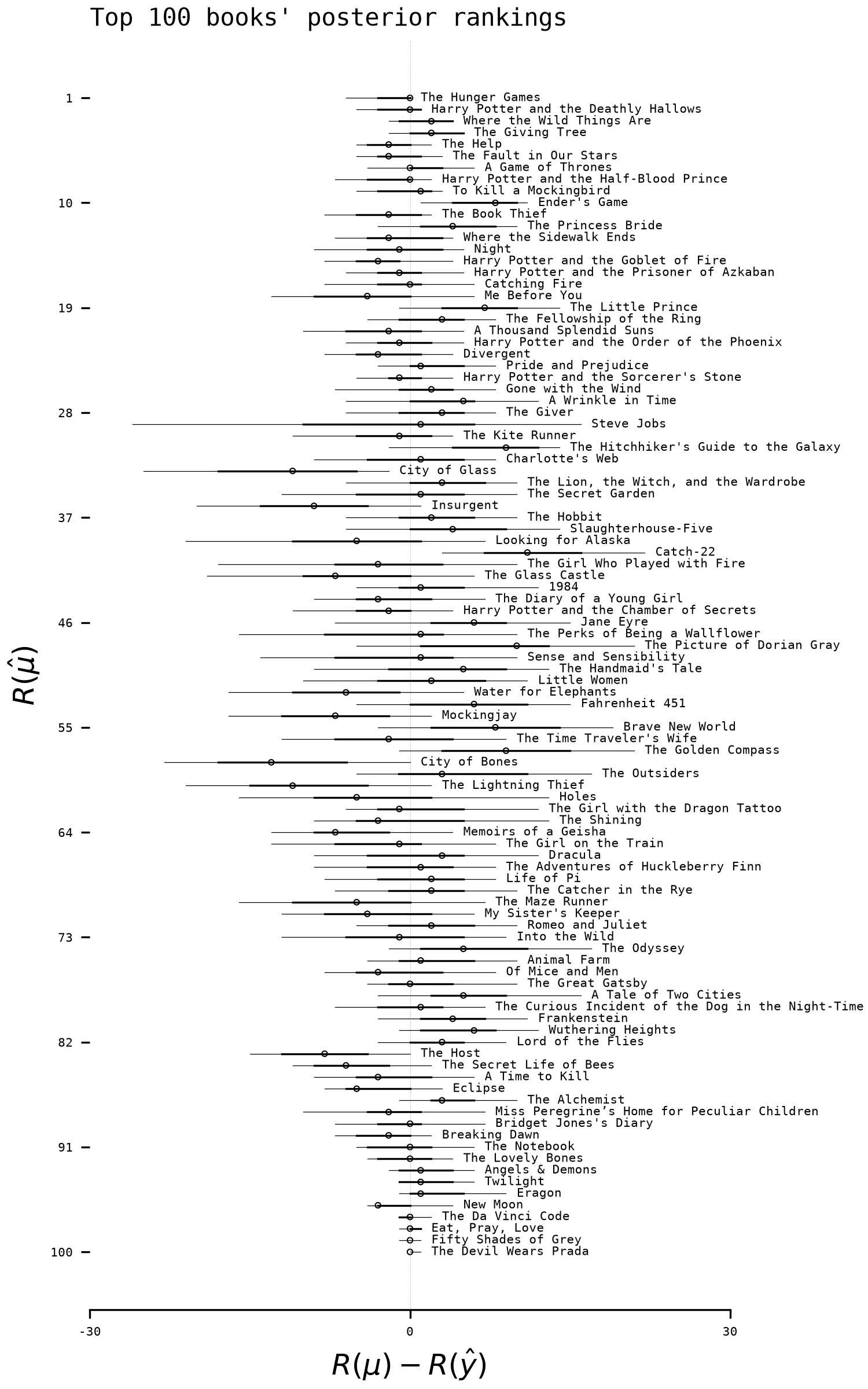
What should you take from this chart? First, that the average posterior rankings often align with the arithmetic means of the user ratings, particularly at the top and bottom of the rankings. The Hunger Games and Harry Potter and the Deathly Hallows are the top-rated books in this sample, and Fifty Shades of Grey and The Devil Wears Prada occupy the 99th and 100th ranks. Second, there is a lot of uncertainty in the rankings of many of the books, such that the distribution of the differences between books could support various inversions in their rankings.
This is perhaps easier to see if we plot the actual latent-scale means, $\hat{\mu}$, against the train-data rankings, $R(\hat{y})$, for each book.
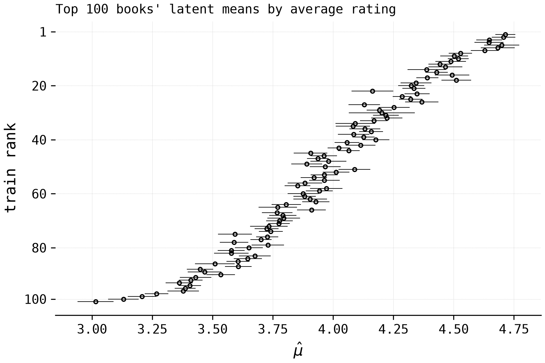
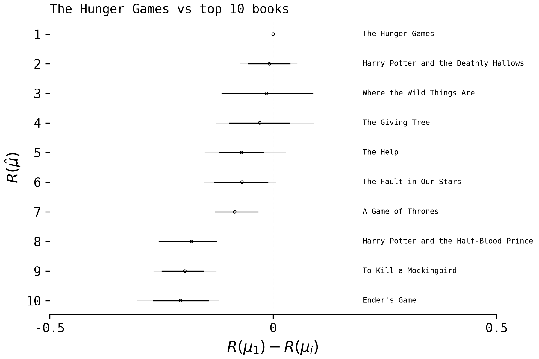
The placement of the means do not form a smooth sigmoid, with horizontal misalignments indicating rank-order differences in the latent scale means compared to the arithmetic mean scores. Even amongst the top ten, the distribution of the differences between books' posterior $\mu$ estimates shows that the top six books' posterior differences include zero, and there is enough uncertainty to plausibly change their rankings.
Posterior predictive distributions
The clear data-generating process of ordinal models make it easy to generate ordinal predictions for each book. Take Jane Eyre, for instance. The plots below show the ordinal ratings against the posterior predictive distributions from each fitted model. The ordinal models show both the mean probabilities (solid circles) of each score with their 95% uncertainty intervals, and 100 samples of their latent scale distribution (pdf lines). The lognormal model shows the lognormal pdf curves only, whilst the Poisson model shows the average probability of each integer (up to 10, but these values are unbounded).
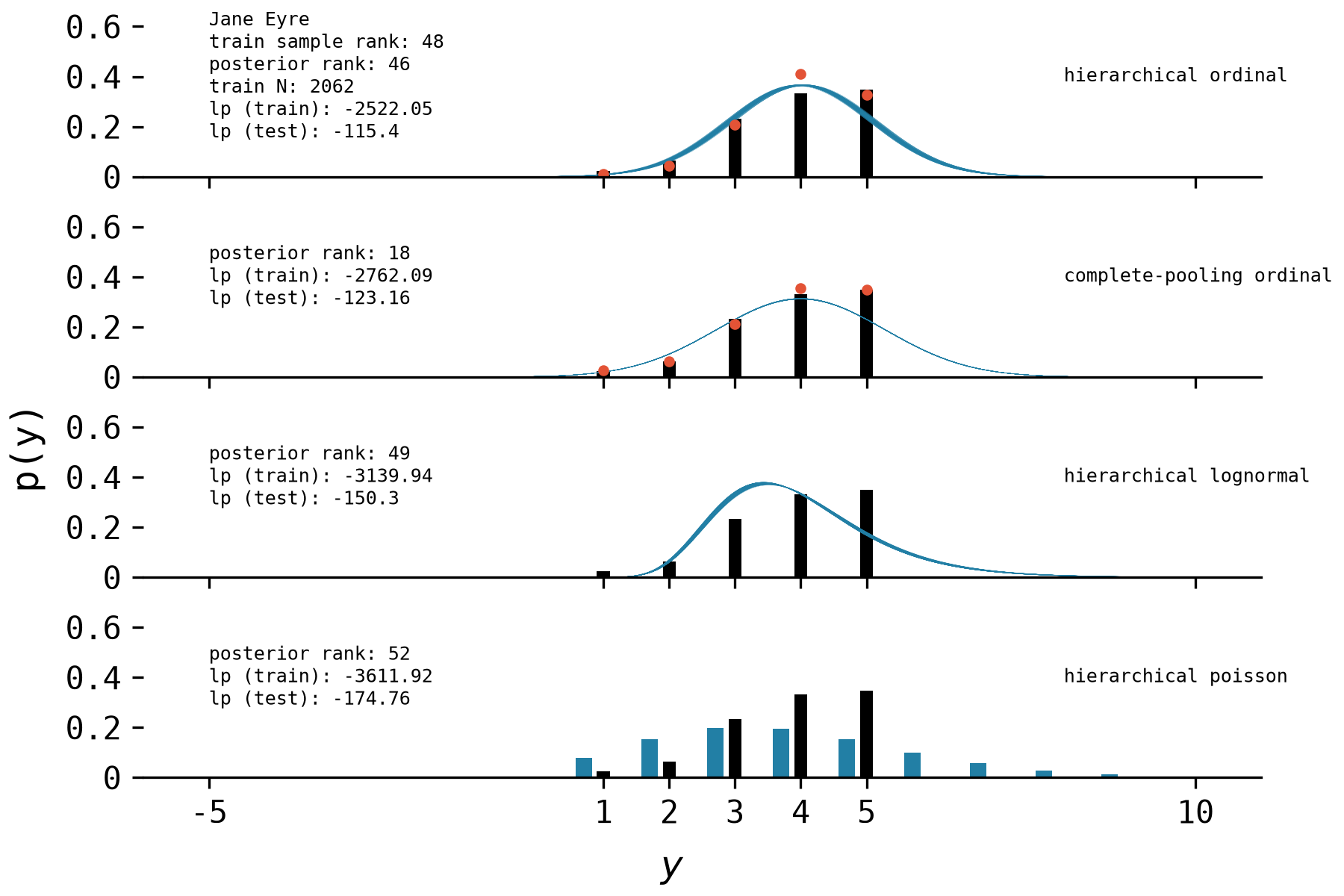
Jane Eyre had over 2k ratings in the training sample, so there was enough data to estimate the parameters with a lot of certainty, which is why you can't detect much difference in the posterior predictive distribution's pdf lines, nor the probabilities of each score. The hierarchical ordinal model does better than the complete pooling ordinal model in-sample and out-of-sample. While the posterior predictive distribution doesn't provide as close a fit to the in-sample data, it better accounts for uncertainty, as the complete pooling model looks too certain. The lognormal model places too much density on lower scores because of its right-skew. Similarly, the Poisson model has infinite positive support, and as a result also places too much mass on the lower ordinal scores, as well as mass on non-existent ordinal categories > 5.
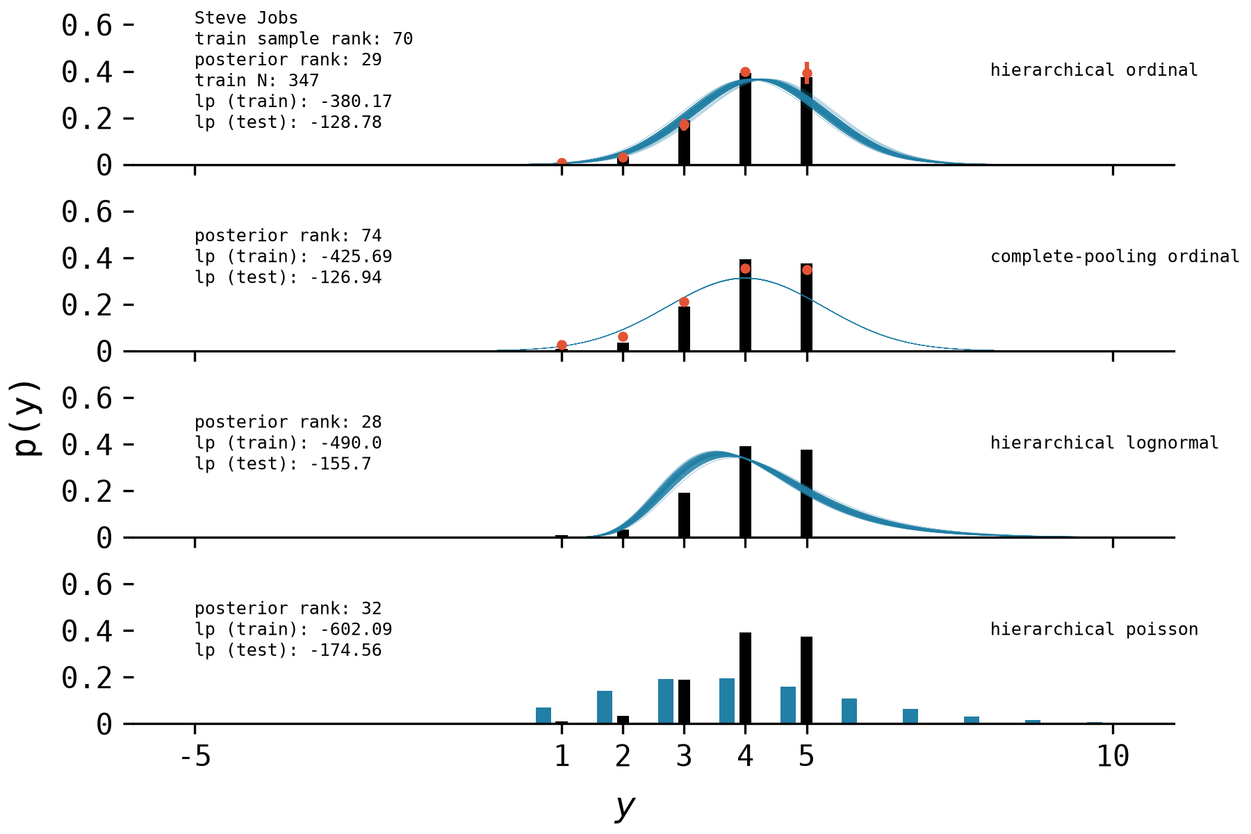
Compare Jane Eyre to the biography Steve Jobs, which only has 347 ratings. Now we can see the uncertainty in the posterior predictive distribution more clearly.
Extensions
There is a wealth of data analysis that could be conducted to improve book rating analytics here. Possible extensions include building models that recommend similar books, perhaps by using something like a Gaussian process over ratings within genres and recommending highly correlated books', or building in measurement error in the ratings, similar to the Dawid-Skene (1979) model. The amount of data here necessitates more efficient inference approaches to be practical, however, since even HMC will take a good while on millions of data points. It could be a cool app idea, however, to provide a place for these type of insights for books.