John Ioannidis' 2005 article Why most published research findings are false is a famous article in the history of 'meta-science'. To some, it is one of the starting places of the reproducibility movement, although many authors raised similar concerns decades previously.
The article focuses on a theoretical model of the publication process and, in particular, the detection of true and false research findings. Many people find the paper and its sentiments interesting but it's use of a mathematical model can make the arguments less accessible to a wider readership. When I was in academia, this article was discussed in local reproducibility network meetings a number of times, and people frequently expressed frustration at not having the time to understand the maths behind the arguments in more detail.
In reality, the mathematical model is simple, which is partly why the paper has received criticism. The model is also Bayesian, which is why I'm interested in it. In this post, I'll repose its main theoretical argument using the language of probability theory rather than medical diagnostic testing and hypothesis testing. I hope this will provide a gentler insight into the paper's findings from first principles. I'm not going to critique the article or delve into the controversies surrounding Ioannidis in recent years.
Table 1
If you understand Table 1 of the paper, you're most of the way there to understanding the mathematical model. Table 1 is a typical contingency table, detailing two discrete events. Along the rows, we can either accept or reject some hypothesis based on running an experiment. Along the columns, the hypothesis is either actually true or false. Each individual cell provides the total number of studies aligning with each of the four outcomes. Of course, in real experiments, you don't know whether a hypothesis was actually true or false, but this is the power of modelling: we make the rules and simulate the process forwards.
Below, we'll consider only the probability of each outcome for ease, but it's often easier to see what's going on with probabilities by starting with frequencies, so here's a simplified Table 1 detailing purely the counts of the different possibilities. Imagine a large number of studies have been run, e.g. 100, with clear accept and reject hypothesis decision criteria, and we can check retrospectively whether the decisions were indeed correct.
| True | False | Total | |
|---|---|---|---|
| Accept | # true accept | # false accept | $\sum$ accept |
| Reject | # false reject | # true reject | $\sum$ reject |
| Total | $\sum$ true | $\sum$ false | $\sum\sum$ |
In the first row, we can either have
true or false accept decisions, and
in the second row we have either
true or false reject decisions.
The former are generally known as
true and false positives, and the latter
as true and false negatives.
The Total row and column
provide the sum of the respective row and
column, and the bottom right cell denotes
the sum of either the total column or
the total row.
To turn this table into a set of probabilities, all we have to do is divide each cell by the total number of studies.
| True | False | Marginal | |
|---|---|---|---|
| Accept | p(a, t) | p(a, f) | p(a) |
| Reject | p(r, t) | p(r, f) | p(r) |
| Marginal | p(t) | p(f) | 1 |
The p() notation here just means "probability of",
and I have initialised the accept/reject and true/false
decisions as lower-case. Note that the bottom right
cell is now known to be 1, because it is the total number of studies
divided by itself, and the Total row/column
has been renamed to Marginal because the
sum of the individual cell probabilities present the
marginal probabilities of the different outcomes.
Think of marginal probabilities as the probability of
an outcome regardless of the other variable.
p(a) is the probability of accepting a hypothesis regardless of whether
it's true or not, p(f) is the probability of a hypothesis being
false regardless of whether the study hypothesis was accepted
or not, and so on.
Marginal probabilities represent an OR logical
relationship. The probability of one event occurring regardless
of any other events (assuming independence) is just a sum of
all the possible way that event could occur. The probability
of wind, regardless of whether it's cloudy or sunny, is
the probability of wind if it's cloudy plus the probability
of wind if it's sunny. More on this below.
If marginal probabilities indicate OR relationships,
each individual cell of the table indicate AND relationships.
Specifically, they are the joint probabilities of two
different events: accept & true, accept & false,
reject & true, and reject & false.
It's the probability of wind and
sun on the same day, or the probability of
wind and cloud.
The marginal probabilities are composed of individual joint probabilities. The probability of wind is the sum of p(wind, cloud) and p(wind, sun). Similarly, the probability of accepting a hypothesis is the sum of p(a, t) and p(a, f), as we can see from the table above. So, what's the joint probability composed of?
If you think logically, the joint probability is composed of two elements. If it's sunny and windy on the same day, that could either occur if it's sunny first, then it's windy, or if it's windy first, then it became sunny. A joint probability can be factored into the probability of one event, alone, multiplied by the probability of the other event given we know the first event has also occurred. The probability of winning a marathon and running under 3 hours is composed of the probability of winning a marathon, regardless of the time, multiplied by the probability of running under 3 hours given winning a marathon. For any events A and B, we have:
p(A, B) = P(A | B) P(B) == P(B | A) P(A)
The 'bar' syntax in p(A | B) is just notation for 'given' or 'conditional on', and therefore these probabilities are simply known as conditional probabilities. Sometimes it's more intuitive to think about conditional probabilities than joint probabilities. If we divide by the marginal probability on both sides of the above equation, we get p(A | B) = p(A, B) / P(B). In words, we can say that the conditional probability is the joint probability corrected for the probability of one of the events. The division focuses our attention on all the possible outcomes to only a subset of possible outcomes, since we already know that one has occurred. The probability of winning a marathon given someone runs under 3 hours automatically limits our attention to all marathon runners who have run under 3 hours. The probability of wind given its raining limits our attention those days it's already raining. If you had historical data on two events in a big Excel sheet, this would be like filtering one column to restrict the attention on a particular outcome.
The definitions of joint, marginal and conditional probabilities are foundational in probability theory, and hold an important concept for understanding Ioannidis' paper. Because of their dependent relationship — the joint factors into the conditional times the marginal, the conditional is the joint divided by the marginal — even if one of those probabilities is particularly high or low, the value of the other could significantly change the outcome. Winning a marathon and running sub-3 hours will probably be rare even if running sub-3 hours is a fast but frequent occurrence for some runners because winning a race is hard. Egypt is one of the driest places on earth, so the chance of if it raining and being windy is still very low even if rain usually follows wind, even in Egypt (I don't know, but you get the point).
This is known as the base rate fallacy,
and is also the reason that complementary conditional probabilities
are not equal. If someone told you they'd won a local marathon,
you'd be pretty sure they ran under 3 hours. But if someone told
you they'd just run under 3 hours for a marathon, you'd probably
be less certain that they'd won, because plenty of others likely
ran under 3 hours too. These are two conditional probabilities,
p(sub-3 | won) and p(won | sub-3),
and their definitions are not equal as long as the marginal
probabilities of winning a marathon and running sub-3 hours
are not equal:
p(sub-3 | won) = p(sub-3, won) / p(won)
p(won | sub-3) = p(sub-3, won) / p(sub-3)

p(sub-3, won) / p(won) > p(sub-3, won) / p(sub-3)
1 > p(won) / p(sub-3)
p(sub-3) > p(won)
Both involve the same joint probability, but because the probability of winning a marathon is quite a bit lower than running sub-3 hours, we'd expect the first conditional probability to be higher than the second. What's important to understand here is that the marginal probability, also known as the base rate or prior probability, matters.
Let's get back to Table 1 of the paper. With these definitions in hand, we can expand the joint probabilities of the simplified table into their conditional and marginal probabilities:
| True | False | Marginal | |
|---|---|---|---|
| Accept | p(a | t) p(t) | p(a | f) p(f) | p(a) |
| Reject | p(r | t) p(t) | p(r | f) p(f) | p(r) |
| Marginal | p(t) | p(f) | 1 |
To save space, I haven't expanded the marginal probabilities, so just remember that these are simply the sum of the rows and/or columns, respectively. This summation is known as the law of total probability.
Table 1 is quite complete, but it doesn't look like the actual Table 1 from the paper. So let's fill in the relevant terms.
The pre-study probability
Ioannidis doesn't use the term 'marginal' or 'base rate' or 'prior' in his paper but calls p(t), the marginal probability of the study being true, the 'pre-study probability' defined using a variable called 'R'. R is the 'odds ratio' of true to false hypotheses, the ratio of p(t) and p(f) in our table above. Rather than talk about probabilities, odds ratios are positive variables but do not have to be between 0 and 1. This is mainly just historical preference, particularly in the field of medical diagnostic testing. Here's what we're told off-the-bat in the paper:
pre-study probability = R / (R + 1)

where R = # true relationships / # false relationships
or    R = p(t) / p(f)
This means that p(t) = R / (R + 1), which can be shown with a bit of long-winded algebra.
p(t) = p(t) / [p(t) + p(f)] # denominator sums to 1
     = p(t) / p(f) * 1 / [p(t) / p(f) + 1]
     = R * 1/(R + 1)
     = R / (R + 1)
The other marginal probability, p(f), is defined as:
p(f) = 1 - p(true)
     = 1 - R/(R + 1)
     = (R + 1) / (R + 1) - R/(R + 1)
     = [(R + 1) - R] / (R + 1)
     = 1 / (R + 1)
p(t) and p(f) sum to 1, as do R / (R + 1) and 1 / (R + 1).
Type 1 and Type 2 errors
Ioannidis also doesn't use the term 'conditional' probability in his paper, but instead uses the more specific terms of Type 1 and Type 2 error rates, which come from the domain of hypothesis testing. A Type 1 error occurs when we accept a hypothesis that is in fact false, and a Type 2 error occurs when we reject a true hypothesis.
Type 1 error = p(a | f) = α
Type 2 error = p(r | t) = β
These two errors are often associated with the Greek letters α and β. Typical values assumed and used for experiment planning in scientific research are α = 0.05 and β = 0.2.
We can nearly fill out our table of probabilities with the terminology and symbols used by Ioannidis, but we still need to obtain p(a | t) and p(r | f). If we look at the definition of marginal probabilities, we can see that conditioning on a variable makes their joint probabilities sum to 1. For instance, for p(f), the marginal probability of the hypothesis being false:
p(f) = p(a, f) + p(r, f)

# divide (condition on) by p(f)
1 = [ p(a, f) + p(r, f) ] / p(f)
  = p(a, f) / p(f) + p(r, f) / p(f)
  = p(a | f) + p(r | f)
So, for the same conditioning variable and two outcomes, we can say that the opposing conditional probability is the complement of the first. As a result, we can define the remaining conditional probabilities directly in terms of α and β.
p(a | t) = 1 - p(r | t)
         = 1 - Type 2 error
         = 1 - β
         = sensitivity

p(r | f) = 1 - p(a | f)
         = 1 - Type 1 error
         = 1 - α
         = specificity
These two conditional probabilities also have their own special names in the diagnostic testing literature: p(a | t) is the sensitivity, the probability of accepting a hypothesis if it's in fact true, and p(r | f) is the specificity, the probability of rejecting a hypothesis if it is in fact false.
Sensitivity is even more widely known as statistical power, and research designs frequently aim for power of at least 80%.
Table 1, defined
We can finally write out Table 1 of the paper using the definitions above to substitute into our table of probabilities. Note, we won't include the $c$ variable, the number of studies, because our table is defined purely in terms of probabilities.
| True | False | Marginal | |
|---|---|---|---|
| Accept | (1 - β) R / (R + 1) | α / (R + 1) | (R + α - R β) / (R + 1) |
| Reject | β R / (R + 1) | (1 - α) / (R + 1) | (β R - α + 1) / (R + 1) |
| Marginal | R / (R + 1) | 1 / (R + 1) | 1 |
Clear as mud? Whilst this model is simple, in the sense that it's just manipulating a few probabilities, the way the paper quickly jumps into the jargon of diagnostic testing and mathematical terms can make it hard to read. Hopefully the slow exposition above has helped someone make better sense about how the terms are derived.
Posterior probability of a true result (PPV)
A key quantity of interest from this paper is the probability that a hypothesis is true given that it's been accepted by an experiment, which is the conditional probability p(t | a). We don't have this probability in our table above you'll notice, and we know that p(t | a) $\neq$ p(a | t) because the marginal probability of p(t) could be very different to p(a).
We can use the fact that joint probabilities are interchangeable to our advantage here by setting them equal to each other and solving for the conditional probability p(t | a).
p(a, t) = p(t, a)
p(a | t) p(t) = p(t | a) p(a)

p(t | a) = p(a | t) p(t) / p(a)
We've just derived a very important rule: Bayes' theorem! Bayes' theorem is simply a way of relating conditional probabilities. We can now use the terms in the table to define this conditional probability:
p(t | a) = (1 - β) R / (R + 1) [(R + 1) / (R + α - R β)]
         = (1 - β) R / (R + α - R β)
This quantity is the 'posterior probability of a true result' or PPV, a common diagnostic in medical testing literature. Ideally, accepting a hypothesis would mean that the hypothesis is in fact true, but that is highly dependent on the base rate or p(t). As we're dealing with probabilities of discrete outcomes, it's helpful to talk about what value p(t | a) would need to obtain to be considered 'true'. One option is to say that p(t | a) should be greater than 50%, which results in the following inequality.
p(t | a) > 0.5
(1 - β) R / [R + α - R β] > 0.5
(1 - β) R > 0.5 * (R + α - R β)
2 (1 - β) R > R + α - R β
2 (1 - β) R > R (1 - β) + α
2 (1 - β) R - R (1 - β) > α
(1 - β) R > α
You can think of this as the 'odds a hypothesis is true'. Ioannidis writes:
Since the vast majority of invesigators depend on a α = 0.05, this means that a research finding is more likely true than false if (1 - β) R > 0.05.
The plot below shows this relationship on the left and the value of p(t | a) (the PPV) on the right for set values of α = 0.05 and two values of β = {0, 0.2}. Setting β to zero means that the Type 2 error, p(r | t), is zero, so that the probability of being true above simply needs to be greater than the Type 1 error rate.
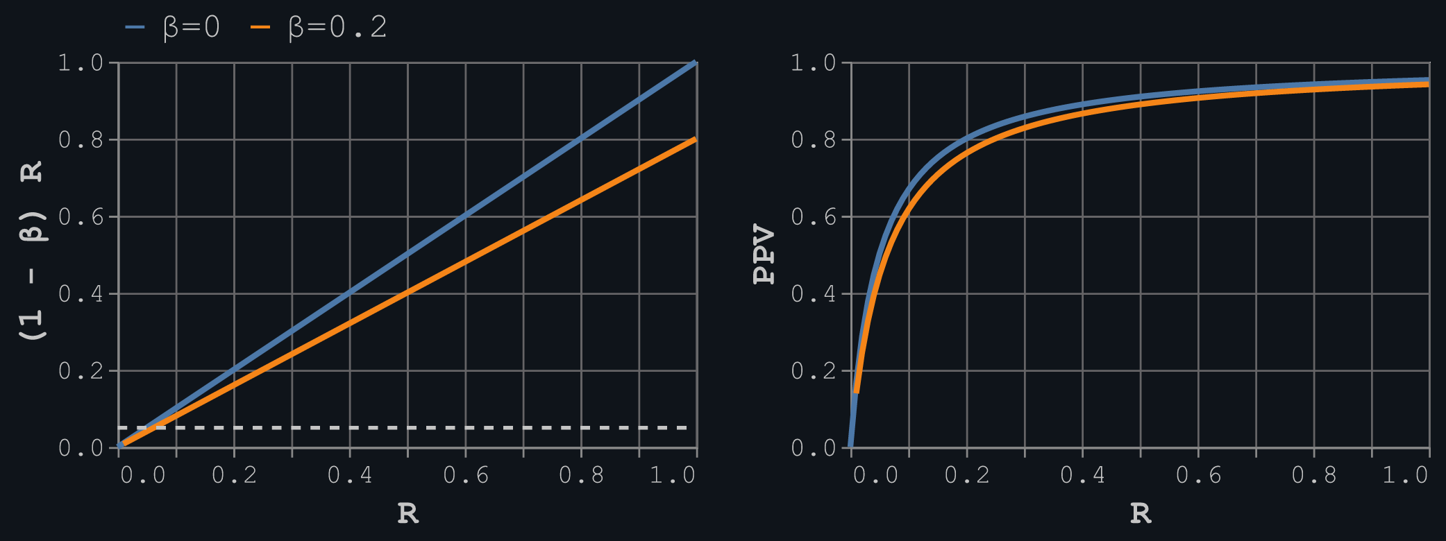
This plot matches results presented in Figure 1 of the paper, with the point being that, for traditional levels of α and 1 - β, and assuming that the pre-study odds or prior probability of a hypothesis being true is probably relatively small, then the chances of an accepted hypothesis actually being true could only be around 50-80%. This actually isn't too bad, but it presents an idealistic view of the publication process. In the model above, we might assume that every study with an accepted hypothesis got there through merit alone, and any false positives or false negatives are down to random fluctuations. But that ignores intentional bias.
Adding bias
The principal analysis in Ioannidis' paper is the addition of how bias changes the results. Specifically, a new decision process is introduced, which is the probability that a hypothesis was rejected but then switched to accepted due to bias. Ioannidis calls this variable 'u'.
u is another conditional probability: the probability a hypothesis is accepted given it was first rejected and its findings manipulated. This could get messy notationally, so I'm going to keep it simple and introduce the term 's' to indicate switching an initial decision due to bias, and 'h' for holding true to an initial decision. Then:
# switch after reject (biased)
p(s | r) = u
# hold after reject (unbiased)
p(h | r) = 1 - u
# switch after accept (never)
p(s | a) = 0
# hold after accept (always)
p(h | a) = 1
Note that we assume people never switch from accept to reject, and always hold onto accept decisions. It's also assumed that these conditional probabilities are independent of the whether the hypothesis is actually true or false.
How does this change our table? Although we now have three events to play with, we can keep the same 2x2 contingency table as before and just update the terms to include the different possibilities. This is a simplified Table 2 from the paper.
| True | False | Marginal | |
|---|---|---|---|
| Accept | p(h, a, t) + p(s, r, t) | p(h, a, f) + p(s, r, f) | p(a) |
| Reject | p(h, r, t) | p(h, r, f) | p(r) |
| Marginal | p(t) | p(f) | 1 |
Each cell is still the joint probability of accepting/rejecting and true/false, but we're now marginalising over the different possible ways that joint probability could arise. Confusingly, it's a joint probability which is also marginal. In reality, all probabilities are marginalising over something because probabilities are always conditioning on other things. We might talk a lot about 'independence' in statistics, but that's an ideal rather than a certainty. The probability of rain, p(rain), is dependent on many of factors, p(rain) = p(rain, factor1) + p(rain, factor2) + ..., etc..
Let's fill out these probabilities. We can break each cell out further into it's component probabilities. I'll just do this for the first column in detail:
p(a, t) = p(h, a, t) + p(s, r, t)
        = p(h | a) p(a | t) p(t) + p(s | r) p(r | t) p(t)
        = 1 (1 - β) R / (R + 1) + u β R / (R + 1)
        = [(1 - β) R + u β R] / (R + 1)

p(r, t) = p(h, r, t) # p(s, a, t) = 0
        = p(h | r) p(r | t) p(t)
        = (1 - u) β R / (R + 1)
Finally, here's Table 2 of the paper re-created. I'm not showing the marginal probabilities of accept and reject, because they'd take up too much space, but you can see the paper for their expressions.
| True | False | |
|---|---|---|
| Accept | [(1 - β)R + uβR] / (R + 1) | [α + u(1 - α)] / (R + 1) |
| Reject | (1 - u)β R / (R + 1) | (1 - u)(1 - α) / (R + 1) |
| Marginal | R / (R + 1) | 1 / (R + 1) |
How do we work out the PPV or p(t | a) in this case? We can once again just use the rules of probability.
p(a, t) = [(1 - β)R + uβR] / (R + 1)

p(a) = [(1 - β)R + uβR + α + u(1 - α)] / (R + 1)

p(t | a) = p(a, t) / p(a)
         = [(1 - β)R + uβR] / [(1 - β)R + uβR + α + u(1 - α)]
The probability that the PPV is at least 50% is also this gnarly expression:
p(t | a) > 0.5
[(1 - β)R + uβR] / [(1 - β)R + uβR + α + u(1 - α)] > 0.5
2 [(1 - β)R + uβR] > (1 - β)R + uβR + α + u(1 - α)
(1 - β)R + uβR > α(1 - u) + u
[R((1 - β) + uβ) - u] / (1 - u) > α
Here's what these relationships look like plotted against the pre-study odds, R, for no bias and a bias of 20%.
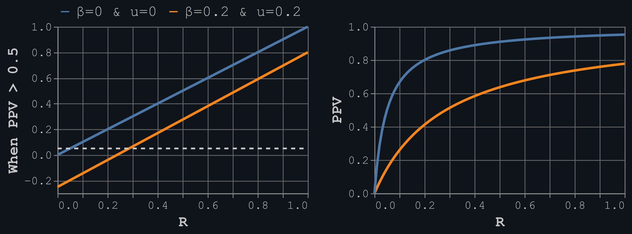
Bias hurts the PPV. The condition on the left shows that we need a pre-study odds greater than 0.3 (1 true to three false hypotheses) to get above the α = 0.05 threshold with a bias of 20%, which aligns with the right plot. You can use the equations to re-create the results in Ioannidis' fourth table of different scenarios, where the chances of getting a PPV > 50% are actually quite difficult. Thus, the probability that a hypothesis is true is < 50% in many cases.
I'll leave it to interested readers to go into further details of Ioannidis' paper and decide on whether its results merit its title. It always surprises me that such a simple exposition of basic probability theory, in what is just a re-hashing of the nearly three-centuries old Bayes' rule, can result in as much notoriety as this paper has received.